Functions and Function Definitions

We shall need a number of mathematical ideas and notations concerning functions in general. Most of the ideas are well known, but the notion of conditional expression is believed to be new², and the use of conditional expressions permits functions to be defined recursively in a new and convenient way.

a. Partial Functions. A partial function is a function that is defined only on part of its domain. Partial functions necessarily arise when functions are defined by computations because for some values of the arguments the computation defining the value of the function may not terminate. However, some of our elementary functions will be defined as partial functions.

b. Propositional Expressions and Predicates. A propositional expression is an expression whose possible values are $T$ (for truth) and $F$ (for falsity). We shall assume that the reader is familiar with the propositional connectives $\land$ (``and''), $\lor$ (``or''), and $\lnot$ (``not''). Typical propositional expressions are:

$$x < y$$

$$(x < y) \land (b = c)$$

x is prime

A predicate is a function whose range consists of the truth values T and F.

c. Conditional Expressions. The dependence of truth values on the values of quantities of other kinds is expressed in mathematics by predicates, and the dependence of truth values on other truth values by logical connectives. However, the notations for expressing symbolically the dependence of quantities of other kinds on truth values is inadequate, so that English words and phrases are generally used for expressing these dependences in texts that describe other dependences symbolically. For example, the function $\vert$x$\vert$ is usually defined in words. Conditional expressions are a device for expressing the dependence of quantities on propositional quantities. A conditional expression has the form

$$(p_1 \rightarrow e_1,\cdots,p_n \rightarrow e_n)$$

where the $p$'s are propositional expressions and the $e$'s are expressions of any kind. It may be read, ``If $p_1$ then $e_1$ otherwise if $p_2$ then $e_2$, $\cdots$ , otherwise if $p_n$ then $e_n$,'' or ``$p_1$ yields $e_1, \cdots , p_n$ yields $e_n$.'' ³

We now give the rules for determining whether the value of

$$(p_1 \rightarrow e_1,\cdots,p_n \rightarrow e_n)$$

is defined, and if so what its value is. Examine the $p$'s from left to right. If a $p$ whose value is $T$ is encountered before any p whose value is undefined is encountered then the value of the conditional expression is the value of the corresponding $e$ (if this is defined). If any undefined $p$ is encountered before a true $p$, or if all $p$'s are false, or if the $e$ corresponding to the first true $p$ is undefined, then the value of the conditional expression is undefined. We now give examples.

$$(1 < 2 \rightarrow 4, 1 > 2 \rightarrow 3) = 4$$

$$(2 < 1 \rightarrow 4, 2 > 1 \rightarrow 3, 2 > 1 \rightarrow 2) = 3$$

$$(2 < 1 \rightarrow 4, T \rightarrow 3) = 3$$

$$(2 < 1 \rightarrow {0 \over 0}, T \rightarrow 3) = 3$$

$$(2 < 1 \rightarrow 3, T \rightarrow {0 \over 0} )\mbox{ is undefined}$$

$$(2 < 1 \rightarrow 3, 4 < 1 \rightarrow 4) \mbox{ is undefined}$$

Some of the simplest applications of conditional expressions are in giving such definitions as

$$\vert x\vert = (x < 0 \rightarrow - x, T \rightarrow x)$$

$$\delta_{ij} = (i = j \rightarrow 1, T \rightarrow 0)$$

$$sgn(x) = (x < 0 \rightarrow - 1, x = 0 \rightarrow 0, T \rightarrow 1)$$

d. Recursive Function Definitions. By using conditional expressions we can, without circularity, define functions by formulas in which the defined function occurs. For example, we write

$$n! = (n = 0 \rightarrow 1, T \rightarrow n \cdot(n - 1)!)$$

When we use this formula to evaluate 0! we get the answer 1; because of the way in which the value of a conditional expression was defined, the meaningless expression 0 $\cdot$ (0 - 1)! does not arise. The evaluation of 2! according to this definition proceeds as follows:

$$\begin{eqnarray*} 2! &=& (2 = 0 \rightarrow 1, T \rightarrow 2 \cdot (2 - 1)!)\\... ...arrow 1, T \rightarrow 0\cdot(0-1)!)\\ &=&2\cdot1\cdot1\\ &=&2 \end{eqnarray*}$$

We now give two other applications of recursive function definitions. The greatest common divisor, gcd(m,n), of two positive integers m and n is computed by means of the Euclidean algorithm. This algorithm is expressed by the recursive function definition:

$$gcd(m,n) = (m > n \rightarrow gcd(n,m), rem(n,m) = 0 \rightarrow m, T \rightarrow gcd(rem(n,m),m))$$

where $rem(n, m)$ denotes the remainder left when $n$ is divided by $m$.

The Newtonian algorithm for obtaining an approximate square root of a number $a$, starting with an initial approximation $x$ and requiring that an acceptable approximation $y$ satisfy $\vert y^2 - a \vert < \epsilon,$ may be written as

sqrt(a, x, $\epsilon$)



= ($\vert x^2 - a\vert < \epsilon \rightarrow$ x,T $\rightarrow$ sqrt (a, ${1 \over 2} (x + {a \over x}), \epsilon))$

The simultaneous recursive definition of several functions is also possible, and we shall use such definitions if they are required.

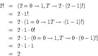
There is no guarantee that the computation determined by a recursive definition will ever terminate and, for example, an attempt to compute n! from our definition will only succeed if $n$ is a non-negative integer. If the computation does not terminate, the function must be regarded as undefined for the given arguments.

The propositional connectives themselves can be defined by conditional expressions. We write

$$\begin{eqnarray*} p \wedge q &=& (p \rightarrow q, T \rightarrow F)\\ p \vee q ... ...htarrow T)\\ p \supset q &=& (p \rightarrow q, T \rightarrow T) \end{eqnarray*}$$

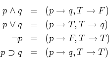
It is readily seen that the right-hand sides of the equations have the correct truth tables. If we consider situations in which $p$ or $q$ may be undefined, the connectives $\wedge$ and $\vee$ are seen to be noncommutative. For example if $p$ is false and $q$ is undefined, we see that according to the definitions given above $p \wedge q$ is false, but $q \wedge p$ is undefined. For our applications this noncommutativity is desirable, since $p \wedge q$ is computed by first computing $p$, and if $p$ is false $q$ is not computed. If the computation for $p$ does not terminate, we never get around to computing $q$. We shall use propositional connectives in this sense hereafter.

e. Functions and Forms. It is usual in mathematics--outside of mathematical logic--to use the word ``function'' imprecisely and to apply it to forms such as $y^2 + x$. Because we shall later compute with expressions for functions, we need a distinction between functions and forms and a notation for expressing this distinction. This distinction and a notation for describing it, from which we deviate trivially, is given by Church [3].

Let $f$ be an expression that stands for a function of two integer variables. It should make sense to write $f(3, 4)$ and the value of this expression should be determined. The expression $y^2 + x$ does not meet this requirement; $y^2 + x(3, 4)$ is not a conventional notation, and if we attempted to define it we would be uncertain whether its value would turn out to be 13 or 19. Church calls an expression like $y^2 + x$, a form. A form can be converted into a function if we can determine the correspondence between the variables occurring in the form and the ordered list of arguments of the desired function. This is accomplished by Church's $\lambda$-notation.

If $\cal E$ is a form in variables $x_1, \cdots, x_n,$ then $\lambda((x_1, \cdots, x_n),\cal E)$ will be taken to be the function of $n$ variables whose value is determined by substituting the arguments for the variables $x_1, \cdots, x_n$ in that order in $\cal E$ and evaluating the resulting expression. For example, $\lambda((x,y),y^2 +x)$ is a function of two variables, and $\lambda((x,y),y^2 +x)(3,4) = 19$.

The variables occurring in the list of variables of a $\lambda$-expression are dummy or bound, like variables of integration in a definite integral. That is, we may change the names of the bound variables in a function expression without changing the value of the expression, provided that we make the same change for each occurrence of the variable and do not make two variables the same that previously were different. Thus $\lambda((x,y),y^2+x),\lambda((u,v), v^2+u)$ and $\lambda((y,x),x^2+y)$ denote the same function.

We shall frequently use expressions in which some of the variables are bound by $\lambda$'s and others are not. Such an expression may be regarded as defining a function with parameters. The unbound variables are called free variables.

An adequate notation that distinguishes functions from forms allows an unambiguous treatment of functions of functions. It would involve too much of a digression to give examples here, but we shall use functions with functions as arguments later in this report.

Difficulties arise in combining functions described by $\lambda$-expressions, or by any other notation involving variables, because different bound variables may be represented by the same symbol. This is called collision of bound variables. There is a notation involving operators that are called combinators for combining functions without the use of variables. Unfortunately, the combinatory expressions for interesting combinations of functions tend to be lengthy and unreadable.

f. Expressions for Recursive Functions. The $\lambda$-notation is inadequate for naming functions defined recursively. For example, using $\lambda$'s, we can convert the definition

$${\rm sqrt}(a,x,\epsilon) = (\vert x^2 - a\vert < \epsilon \r... ...ightarrow {\rm sqrt}(a, {1 \over 2}(x + {a \over x}),\epsilon))$$

into

$${\rm sqrt} = \lambda((a,x,\epsilon),(\vert x^2 - a\vert < \ep... ...tarrow {\rm sqrt} (a,{1 \over 2}(x + {a \over x}), \epsilon))),$$

but the right-hand side cannot serve as an expression for the function because there would be nothing to indicate that the reference to $sqrt$ within the expression stood for the expression as a whole.

In order to be able to write expressions for recursive functions, we introduce another notation. $label(a,\cal E)$ denotes the expression $\cal E$, provided that occurrences of $a$ within $\cal E$ are to be interpreted as referring to the expression as a whole. Thus we can write

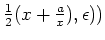
label(sqrt, $\lambda((a,x,\epsilon),(\vert x^2 - a\vert < \epsilon \rightarrow x, T \rightarrow {\rm sqrt} (a, {1 \over 2}(x + {a \over x}),\epsilon))))$

as a name for our sqrt function.

The symbol $a$ in label ($a,\cal E$) is also bound, that is, it may be altered systematically without changing the meaning of the expression. It behaves differently from a variable bound by a $\lambda$, however.